


Working with new data can be overwhelming. How do you extract information and knowledge from the facts sitting in front of you? In this article, we’ll explore a new dataset. We’ll ask, then answer, a number of common types of questions. Exercises and the full dataset are available for those who want to dig deeper.
Cast yourself back to a simpler time… when the web was new and filled with possibilities — August, 1995. Personally, I was just settling into my first weeks of university, where for the first time, I had a direct connection to the internet. After years of 10¢/min long-distance dial-up America Online, I was finally free to surf the world-wide-web without restriction. Oh what a time to be alive.
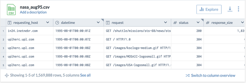
One of the sites I distinctly recall visiting in those first weeks was NASA.gov. They were one of a handful of agencies who embraced the web in those days. Ironically, I recently came across something interesting… a dataset of server logs… from August of ‘95!

requsting_host: the originating host of the requestdatetime: The date and time of the requestrequest: Info about the requested resource (GET/POST, path, HTTP version)status: Response status (200 ok, 404 not found, 5xx error, 30x redirect)size: Size of the response
I’ve uploaded this file to data.world/shad/nasa-website-data for further analysis with SQL.
Now, let’s consider what sorts of questions we might have asked of this data had we worked with NASA more than 20 years ago.
“What’s the most popular time of day for visitors?”
I was pretty active in the 10pm — 2am timeframe, but perhaps this wasn’t typical. Let’s see…

DATE_PART() is a great way to work with dates. It allows us to isolate individual parts of a date. In this case, we’ve isolated the hour of the day and aggregated (using GROUP BY).
Looks like midday is the highest traffic time of day, with significantly less traffic during the night. Not entirely surprising I suppose, but interesting nonetheless.
“What’s the most popular day of the week?”
This is nearly the same question as before, only on a different part of the date, namely the day of the week. We can simply adjust our query from before, changing the DATE_PART() from “hour” to “dayofweek”.

Now we have all of our traffic aggregated to the day of the week when the request was made. Day 4 (Thursday) is the largest day for traffic, followed closely by 2 (Tuesday). Weekends were a significantly slower.
Now, let’s think about traffic a bit more generally. Perhaps there was a specific Thursday that was popular for some reason. Let’s dig a bit deeper and look at each week to see how traffic compares.
“Did we have more traffic at the beginning of the month, or the end?”
In this case, we want to see how weeks compare to one another. We could simply sum up the total count of requests, but we have a partial weeks in our data, so we can’t directly compare totals. What we actually need to see is the average number of requests per day for each week of our data (including partial weeks). This allows us to compare weeks and see how our traffic changes over time.

Here we introduce a new concept — the WITH subquery. Subqueries allow us to create temporary tables that exist only for the duration of a query. This is useful for breaking up complex queries into understandable chunks. In this case, we first create a table, days, which contains the date and count of requests.
Next, we use the days table and aggregated it by week. Note that the week number isn’t very interesting (1–52) so we instead select the minimum date as the start_of_week. We’re also calculating the average number of events per day, and for good measure, we’ll include the distinct number of days contained in the week.
We now have a clear picture of when we were receiving traffic during the month, but perhaps we would like to know where the traffic is coming from.
“What was the most popular domain traffic was requested from?”
Let’s take a step back from dates and consider the requesting_host.

Here again we’ve done a simple aggregation on the host and calculated the number of requests.
But this result has some issues. Many of these hosts appear to be the similar. Hosts such as piweba3y.prodigy.com and piweba5y.prodigy.com should probably be collapsed into a single row. Let’s clean these up by stripping off the prefixes prior to aggregating.

This query introduces the REPLACE() function, which takes a column and uses a regular expression to find some text, and replace it (in this case, with an empty string). Regular expressions may seem complicated at first, but they’re extremely powerful when cleaning up data.
This regular expression above reads (roughly)…
^              Start at the beginning of the string
(              Start group
  gw\d+       “gw”, followed by 1+ numeric digits
  |            OR
www.*proxy   “www”, then 0+ chars followed by “proxy”
  |            OR
  piweb[^.]+   “piweb” followed by 1+ chars that are NOT a period
)              End Group
\.            Followed by a period
If this regular expression matches some part of the requesting_host, then we will replace with the empty string. This allows us to group more effectively.
The majority of traffic appears to come from aol.com and prodigy.com. This was hidden from us before, but now it’s really clear.
Exercise: Can you improve this regular expression to be more generic?
Get Started
HINT: Search online for “Regex Lookahead”.
Give up? Here is a version that leaves onlyhost.com.
“What were the most popular pages?”
This is a common sort of question that you’ll receive—which page is performing the best.

In this query, we’re filtering out images since we really want to just focus on pages of data. (Images are loaded on multiple pages, so pollute the data quite a bit). We’re also stripping off HTTP/1.0 since we don’t care about that for this query.
From this, it’s pretty clear that nasa.gov/ksc.html was the most popular page during the course of this month — even more popular than the root domain page nasa.gov/. That’s interesting, but was it the most popular page on multiple days of the month?

Here we’re first calculating the number of requests going to each page on each day. We’re then aggregating to the day level and using some advanced functions to select just the bits of data we want. MAX() is function to select the maximum value from within the group. MAX_BY() is similar, but uses the max value to select values from other fields on the same row. The combination allows us to find the page that had the maximum number of requests per day of the month.
As you can see, on days where it was popular, it was very popular.
Exercise: Find out how many page views
/ksc.htmlhas each day of the month to see if there’s a pattern. Get Started
Next, I’m interested in that size field. Let’s dig into that a bit and see what we can find.
“What domain/ip requested the most data?”

Here we’re introducing a new aggregation function, SUM(). This allows us to sum up all of the requested bytes within the group. Now we can compare domains to see which is requesting the most data from our servers.
Perhaps unsurprisingly, these domains are similar to the list from before — more requests means more bytes downloaded. What we should probably do is calculate the average number of bytes per domain instead of the total. I will leave this as an exercise for the reader.
Exercise: Which domain requested the largest average amount of data per day over the course of the month? Get Started
Exercise: What was the largest file downloaded by each domain during the month? Get Started
Exercise: Read up on Aggregations and Aggregation Functions and see what else you can find in this data!
“Finally, were there any requests from my university?”
I started this journey in a dorm room back in August of ’95. Seems only fitting that we ask “Are my requests captured here?”

Looks like there was about 13mb of data downloaded to servers at vt.edu.
Exercise: Did alum from your alma mater hit NASA.gov in August ‘95? Replace “vt.edu” with the domain of your choice and find out! Get Started
Obviously, there probably isn’t much value in digging through 20 year old server logs. There is value, however, in understanding the tools and methods for aggregating and filtering data. My hope is that you’re now prepared to take these examples and apply them to your own questions. Whether you’re dealing with time series requests, analytics data, or financial transactions, these same methods can be applied to your data.
Want to dig into NASA server logs a bit more? The full dataset is available on data.world. Feel free to explore and query this data as much as you want. Don’t worry, you won’t break it!
Have your own data that you’d like to explore? Create an account on data.world, create a new dataset, and test out your SQL chops. It’s quick, easy and secure.
Learn more in our SQL Docs, or check out our webinar where we discuss some of these topics in more detail.
